
Linear Regression From Scratch
Linear regression (single variable) begins with this:
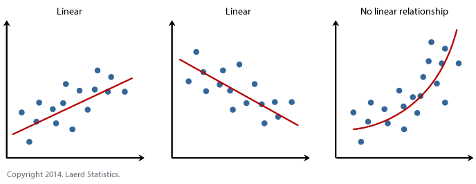
- We have a feature variable (X) and a target variable (y) that have a linear relationship.
 [https://statistics.laerd.com/spss-tutorials/linear-regression-using-spss-statistics.php]
- Imagine the dataset is the transaction history of a freelance developer. Your bread and butter is machine learning, not freelance web dev, so you just want to pay someone to get the job done.
- Our goal is to “LEARN” where to put that red line, such that when we ingest a new X data point, we can predict y with minimal error. In other words, when we know how much time it will take, we can predict how much the job will cost.
- We hope to have a hypothesis/prediction equation that looks like this: \(\hat{y} = wx + b\) \(\text{where } w = weight, b = bias\)
- given x, number of hours, we predict y, the cost of the project
Our cost function is as follows: \(MSE = \frac{1}{N} \sum_{i=1}^n (y_i - (wx_i+b))^2 \\ J(w, b) = \frac{1}{N} \sum_{i=1}^n (y_i - (wx_i+b))^2\)
Looking at it closely:
- $(y_i - (wx_i+b))$ is the difference between the true $y$ value at the $i^{th}$ spot and the predicted value (given the weight and bias).
- This value is summed up across the $n$ datapoints and then divided by the number of datapoints, hence “mean square error”
- We want to minimize that Mean Square Error so that our predicted linear regression line is as close as possible to the real values
Now we need a search algorithm that can find $w,b$ such that $J$ is minimized. We can use gradient descent. Gradient descent chooses initial values for $w$ and $b$ and then repeatedly performs an update until the cost funciton is minimized. The reason why it is called gradient descent, is because we take the gradient of $J$ and then use the corresponding derivatives in the update rule. I’ll update this with the more explanation on gradient descent, partial derivatives, and whatever else to make it more thorough.
def predict(x, weight, bias):
    return (weight*x + b)

def mse_cost(x, y, weight, bias):
    error = 0.0
    for i in range(len(x)):
        error += (y[i] - (weight*x[i]+bias))**2
    return error/len(x)

def grad_desc_update(x, y, weight, bias, alpha):
    d_weight = 0.0 # initialize at 0
    d_bias = 0.0 # initialize at 0

    for i in range(len(x)):
        d_weight += -2*x[i] * (y[i] - (weight*x[i] + bias))
        d_bias += -2*(x[i] - (weight*x[i] + bias))

    weight -= (d_weight / len(x)) * alpha
    bias -= (d_bias / len(x)) * alpha

    return weight, bias

def train(x, y, weight, bias, alpha, iterations):

    for i in range(iterations):
        weight,bias = grad_desc_update(x, y, weight, bias, alpha)

        cost = mse_cost(x, y, weight, bias)

        if i % 10 == 0:
            print("iteration: {}, cost: {}".format(i, cost))

    return weight, bias
Let’s generate some fake data:
def generate_linear_data(x):
    m = 0.014
    b = 0.52
    y = [x_i*m+b+random.random() for x_i in x]
    return np.array(y)


x = list()
for i in range(100):
    x.append(random.randint(0, 100))

x = np.array(x)

y = generate_linear_data(x)
Then try for yourself:
weight, bias = train(x, y, weight=0.0, bias=0.0, alpha=0.001, iterations=100)