Linear Regression From Scratch
Linear regression (single variable) begins with this:
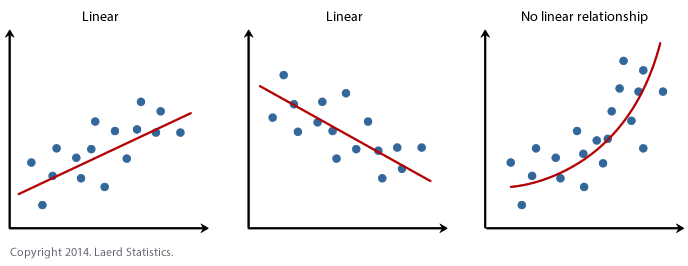
- We have a feature variable (X) and a target variable (y) that have a linear relationship.
 [https://statistics.laerd.com/spss-tutorials/linear-regression-using-spss-statistics.php]
- Imagine the dataset is the transaction history of a freelance developer. Your bread and butter is machine learning, not freelance web dev, so you just want to pay someone to get the job done.
- Our goal is to “LEARN” where to put that red line, such that when we ingest a new X data point, we can predict y with minimal error. In other words, when we know how much time it will take, we can predict how much the job will cost.
- We hope to have a hypothesis/prediction equation that looks like this: \(\hat{y} = wx + b\) \(\text{where } w = weight, b = bias\)
- given x, number of hours, we predict y, the cost of the project
Our cost function is as follows: \(MSE = \frac{1}{N} \sum_{i=1}^n (y_i - (wx_i+b))^2 \\ J(w, b) = \frac{1}{N} \sum_{i=1}^n (y_i - (wx_i+b))^2\)
Looking at it closely:
- $(y_i - (wx_i+b))$ is the difference between the true $y$ value at the $i^{th}$ spot and the predicted value (given the weight and bias).
- This value is summed up across the $n$ datapoints and then divided by the number of datapoints, hence “mean square error”
- We want to minimize that Mean Square Error so that our predicted linear regression line is as close as possible to the real values
Now we need a search algorithm that can find $w,b$ such that $J$ is minimized. We can use gradient descent. Gradient descent chooses initial values for $w$ and $b$ and then repeatedly performs an update until the cost funciton is minimized. The reason why it is called gradient descent, is because we take the gradient of $J$ and then use the corresponding derivatives in the update rule. I’ll update this with the more explanation on gradient descent, partial derivatives, and whatever else to make it more thorough.
1
2
3
4
5
6
7
8
9
10
11
12
13
14
15
16
17
18
19
20
21
22
23
24
25
26
27
28
29
30
31
32
33
def predict(x, weight, bias):
    return (weight*x + b)

def mse_cost(x, y, weight, bias):
    error = 0.0
    for i in range(len(x)):
        error += (y[i] - (weight*x[i]+bias))**2
    return error/len(x)

def grad_desc_update(x, y, weight, bias, alpha):
    d_weight = 0.0 # initialize at 0
    d_bias = 0.0 # initialize at 0

    for i in range(len(x)):
        d_weight += -2*x[i] * (y[i] - (weight*x[i] + bias))
        d_bias += -2*(x[i] - (weight*x[i] + bias))

    weight -= (d_weight / len(x)) * alpha
    bias -= (d_bias / len(x)) * alpha

    return weight, bias

def train(x, y, weight, bias, alpha, iterations):

    for i in range(iterations):
        weight,bias = grad_desc_update(x, y, weight, bias, alpha)

        cost = mse_cost(x, y, weight, bias)

        if i % 10 == 0:
            print("iteration: {}, cost: {}".format(i, cost))

    return weight, bias
Let’s generate some fake data:
1
2
3
4
5
6
7
8
9
10
11
12
13
14
def generate_linear_data(x):
    m = 0.014
    b = 0.52
    y = [x_i*m+b+random.random() for x_i in x]
    return np.array(y)


x = list()
for i in range(100):
    x.append(random.randint(0, 100))

x = np.array(x)

y = generate_linear_data(x)
Then try for yourself:
1
weight, bias = train(x, y, weight=0.0, bias=0.0, alpha=0.001, iterations=100)